Shipping Your NLP Sentiment Classification Model With Confidence

This code-along walks through ingesting embedding data and looking at embedding drift

October 13, 2022

Francisco Castillo

This code-along walks through ingesting embedding data and looking at embedding drift.

This blog was written in partnership with Nate Mar, Founding Engineer at Arize
by Francisco Castillo Carrasco

Increasingly, companies are turning to natural language processing (NLP) sentiment classification to better understand and improve customer experience. From call centers to loyalty programs, these models inform important business decisions across a wide variety of customer touch-points. Unfortunately, many ML teams today do not have reliable ways to monitor these models in production and stay on top of things like embedding drift. This post is designed to help them get started.

Let’s say you are in charge of maintaining a sentiment classification model. This simple model takes online reviews of products from your U.S.-based store as the input and predicts whether the reviewer’s sentiment is positive, negative, or neutral. You trained your sentiment classification model on English reviews. However, once the model was released into production, your colleagues start to notice that the performance of the model has degraded over a period of time.

Monitoring is critical to surfacing the reason for this performance degradation. In this example, maybe a sudden influx of reviews written in Spanish impacts the model’s performance. You can surface and troubleshoot this issue by analyzing the embedding vectors associated with the online review text. By inspecting embedding drift, you can also surface problems with your data before it causes performance degradation.

This blog covers how to start from scratch. We will:

Download the data
Preprocess the data
Train the model
Extract embedding vectors and predictions
Log the inferences

For the purposes of this example, we will be using Hugging Face’s open source libraries and Arize for monitoring (full disclosure: I work for Arize).

In particular, we will use:

Datasets: a library for easily accessing and sharing datasets and evaluation metrics for Natural Language Processing (NLP), computer vision, and audio tasks.
Transformers: a library to easily download and use state-of-the-art pre-trained models. Using pre-trained models can lower your compute costs, reduce your carbon footprint, and save you time from training a model from scratch.
Monitoring: if this is your first time with Arize, it’s worth signing up for a free account or consulting this tutorial on sending data before continuing.

Let’s get started!

Step 0: Setup and Getting the Data

The preliminary step is to install datasets and transformers libraries mentioned above. In addition, we will import some metrics from scikit-learn.

We’ll explain each of the imports below as we use them.

Install Dependencies and Import Libraries 📚

!pip install -q datasets transformers arize

import pandas as pd

import torch

from datasets import load_dataset

from transformers import AutoTokenizer, AutoModelForSequenceClassification, Trainer, TrainingArguments

from sklearn.metrics import accuracy_score, f1_score

from datetime import datetime

import uuid

from arize.pandas.logger import Client

from arize.utils.types import Environments, ModelTypes, EmbeddingColumnNames, Schema

Check if GPU Is Available

Here we use Pytorch to check whether a GPU is available or not. When appropriate we will use PyTorch’s nn.Module.to() method to ensure that the model will run on the GPU if we have one.

device = torch.device("cuda" if torch.cuda.is_available() else "cpu")

🌐 Download the Data

The easiest way to load a dataset is from the Hugging Face Hub. There are already thousands of datasets in over 100 languages on the Hub. At Arize, we have crafted the arize-ai/ecommerce_reviews_with_language_drift dataset for this example notebook.

Thanks to Hugging Face 🤗 datasets, we can download the dataset in one line of code. The Dataset object comes equipped with methods that make it very easy to inspect, pre-process, and post-process your data.

dataset = load_dataset("arize-ai/ecommerce_reviews_with_language_drift")

train_ds = dataset["training"]

val_ds = dataset["validation"]

prod_ds = dataset["production"]

Inspect the Data

It is often convenient to convert a Dataset object to a Pandas DataFrame so we can access high-level APIs for data visualization. 🤗 Datasets provides a set_format() method that allows us to change the output format of the Dataset. This does not change the underlying data format, an Arrow table. When the DataFrame format is no longer needed, we can reset the output format using reset_format().

train_ds.set_format("pandas")

display(train_ds[:].head())

train_ds.reset_format()

Step 1: Developing Your Sentiment Classification Model

Pre-Processing the Data

Before being able to input the data into the model for fine-tuning, we need to perform an important step: tokenization.

Transformer models like DistilBERT cannot receive raw strings as input. We need to tokenize and encode the text as numerical vectors. We will perform Subword Tokenization, which is learned from the pre-training corpus. Its goal is to allow tokenization of complex words (or misspellings) into smaller units that the model can learn, and keep common words as unique entities, keeping the length of the input to a reasonable size.

Hugging Face Transformers provides the AutoTokenizer class, which allows us to quickly download the tokenizer required by the pre-trained model of our choosing.

In this case, we will use the following checkpoint: distilbert-base-uncased.

model_ckpt = "distilbert-base-uncased"

tokenizer = AutoTokenizer.from_pretrained(model_ckpt)

Next, let’s define a processing function to tokenize the examples in the dataset. The padding and truncation options are added to keep the inputs to a consistent length. Shorter sequences are padded and longer ones are truncated. We can apply said processing function to entire dataset objects by using the map() method.

def tokenize(batch, max_length=512):

return tokenizer(batch['text'], padding=True, truncation=True, max_length=max_length)

process_batch_size = 100

max_size = 100 # max length of the tokenized sequence

train_ds = train_ds.map(lambda batch: tokenize(batch, max_size), batched=True, batch_size=process_batch_size)

val_ds = val_ds.map(lambda batch: tokenize(batch, max_size), batched=True, batch_size=process_batch_size)

prod_ds = prod_ds.map(lambda batch: tokenize(batch, max_size), batched=True, batch_size=process_batch_size)

Two columns have appeared in each dataset:

input_ids: A numerical identifier to which each token has been mapped.
attention_mask: Array of 1s and 0s, allowing the model to ignore the padded parts of the inputs.

We can display the dataset changes as it was shown above:

train_ds.set_format("pandas")

display(train_ds[:].head())

train_ds.reset_format()

Build the Model

Similar to how we obtained the tokenizer, Hugging Face Transformers provides the AutoModelForSequenceClassification class, which allows us to quickly download a pre-trained transformer model with a classification task head on top. The pre-trained model to use in this tutorial is DistilBERT. The weights of the classification task head will be randomly initialized.

It is important to pass output_hidden_states = True to be able to compute the embedding vectors associated with the text (explained below). First, let’s download the pre-trained model.

num_labels = dataset['training'].features['label'].num_classes

model = (AutoModelForSequenceClassification

.from_pretrained(model_ckpt, num_labels = num_labels, output_hidden_states=True)

.to(device))

We then use the TrainingArugments class to define the training parameters. This class stores a lot of information and gives you control over the training and evaluation.

training_batch_size = 16

training_epochs = 3

logging_steps = len(train_ds) // training_batch_size

model_name = f"distilbert_reviews_with_language_drift"

training_args = TrainingArguments(output_dir=model_name,

num_train_epochs=training_epochs,

learning_rate=2e-5,

per_device_train_batch_size=training_batch_size,

per_device_eval_batch_size=training_batch_size,

weight_decay=0.01,

evaluation_strategy="epoch",

disable_tqdm=False,

logging_steps=logging_steps,

log_level="error",

optim="adamw_torch"

)

Next, define a metrics calculation function to evaluate the model.

def compute_metrics(pred):

labels = pred.label_ids

preds = pred.predictions[0].argmax(-1)

f1 = f1_score(labels, preds, average="weighted")

acc = accuracy_score(labels, preds)

return {"accuracy": acc, "f1": f1}

Finally, fine-tune the model using the Trainer class.

trainer = Trainer(

model=model,

args=training_args,

compute_metrics=compute_metrics,

train_dataset=train_ds,

eval_dataset=val_ds,

tokenizer=tokenizer,

)

print("Evaluation before training")

eval = trainer.evaluate(eval_dataset=val_ds)

eval_df = pd.DataFrame({'Epoch':0, 'Validation Loss': eval['eval_loss'], 'Accuracy': eval['eval_accuracy'], 'F1': eval['eval_f1']}, index=[0])

display(eval_df)

print(" ")

torch.cuda.empty_cache() # Free up some memory

print("\nTraining...")

trainer.train()

Step 2: Post-Processing Your Data

Here, we will extract the prediction labels and the text embedding vectors. The latter are formed from the hidden states of the pre-trained (and then fine-tuned) model.

def postprocess(batch):

"""

Postprocessing includes:

- Extract prediction labels

- Extract embedding vectors associated with the input text

"""

inputs = {k:v.to(device) for k,v in batch.items() if k in tokenizer.model_input_names}

with torch.no_grad():

out = model(**inputs). # Extract prediction labels

pred_label = out.logits.argmax(dim=1) # Extract embedding vectors

hidden_states = torch.stack(out.hidden_states) # (layer_#, batch_size, seq_length/or/num_tokens, hidden_size)

embeddings = hidden_states[-1][:,0,:] # Select last layer, then CLS token vector

return {"text_vector": embeddings.cpu().numpy(), "pred_label": pred_label.cpu().numpy()}

train_ds.set_format("torch", columns=["input_ids", "attention_mask"])

train_ds = train_ds.map(postprocess, batched=True, batch_size=process_batch_size)

val_ds.set_format("torch", columns=["input_ids", "attention_mask"])

val_ds = val_ds.map(postprocess, batched=True, batch_size=process_batch_size)

prod_ds.set_format("torch", columns=["input_ids", "attention_mask"])

prod_ds = prod_ds.map(postprocess, batched=True, batch_size=process_batch_size)

Step 3: Prepare Your Data To Be Sent for Monitoring

From this point forward, it is convenient to use Pandas DataFrames. This can be done easily using the format methods already covered.

train_df = train_ds.to_pandas()

val_df = val_ds.to_pandas()

prod_df = prod_ds.to_pandas()

Update the Timestamps

The data that you are working with was constructed in April of 2022. Hence, we will update the timestamps so they are current at the time that you’re sending data to Arize.

last_ts = max(prod_df['prediction_ts'])

now_ts = datetime.timestamp(datetime.now())

delta_ts = now_ts - last_ts

train_df['prediction_ts'] = (train_df['prediction_ts'] + delta_ts).astype(float)

val_df['prediction_ts'] = (val_df['prediction_ts'] + delta_ts).astype(float)

prod_df['prediction_ts'] = (prod_df['prediction_ts'] + delta_ts).astype(float)

Map Labels To Class Names

We want to log the inferences with the corresponding class names (for predictions and actuals) instead of the numeric label. Since we used 🤗 Datasets to download the dataset, it came equipped with methods to do this.

The dataset we downloaded defined the label to be an instance of the datasets.ClassLabel class, which has the convenient method int2str (visit Hugging Face documentation for more information).

def label_int2str(row):

return train_ds.features['label'].int2str(row)

train_df['label'] = train_df['label'].apply(label_int2str)

val_df['label'] = val_df['label'].apply(label_int2str)

prod_df['label'] = prod_df['label'].apply(label_int2str)

train_df['pred_label'] = train_df['pred_label'].apply(label_int2str)

val_df['pred_label'] = val_df['pred_label'].apply(label_int2str)

prod_df['pred_label'] = prod_df['pred_label'].apply(label_int2str)

Add Prediction IDs

The Arize platform uses prediction IDs to link a prediction to an actual. Visit the Arize documentation for more details. You can generate prediction IDs as follows:

def add_prediction_id(df):

return [str(uuid.uuid4()) for _ in range(df.shape[0])]

train_df['prediction_id'] = add_prediction_id(train_df)

val_df['prediction_id'] = add_prediction_id(val_df)

prod_df['prediction_id'] = add_prediction_id(prod_df)

Step 4: Sending Data Into Arize 💫

The first step is to set up the Arize client. After that we will log the data.

Import and Setup Client

Copy the Arize API_KEY and SPACE_KEY from your Space Settings page (shown below) to the variables in the cell below. We will also be setting up some metadata to use across all logging.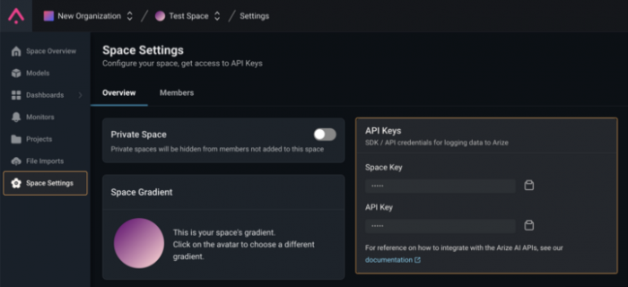

SPACE_KEY = "SPACE_KEY"

API_KEY = "API_KEY"

arize_client = Client(space_key=SPACE_KEY, api_key=API_KEY)

model_id = "NLP-demo-sentiment-classification-language-drift"

model_version = "1.0"

model_type = ModelTypes.SCORE_CATEGORICAL

if SPACE_KEY == "SPACE_KEY" or API_KEY == "API_KEY":

raise ValueError("❌ NEED TO CHANGE SPACE AND/OR API_KEY")

else:

print("✅ Import and Setup Arize Client Done! Now we can start using Arize!")

Now that our Arize client is setup, let’s go ahead and log all of our data to the platform. For more details on how arize.pandas.logger works, visit our documentation.

Define the Schema

A Schema instance specifies the column names for corresponding data in the DataFrame. While we could define different Schemas for training and production datasets, the DataFrames have the same column names, so the Schema will be the same in this instance.

To ingest non-embedding features, it suffices to provide a list of column names that contain the features in our DataFrame. Embedding features, however, are a little bit different.

Arize allows you to ingest not only the embedding vector, but the raw data associated with that embedding, or a URL link to that raw data. Therefore, up to three columns can be associated to the same embedding object*. To be able to do this, Arize’s SDK provides the EmbeddingColumnNames class, used below.

*NOTE: This is how we refer to the 3 possible pieces of information that can be sent as embedding objects:

Embedding vector (required)
Embedding data (optional): raw text associated with the embedding vector
Embedding link_to_data (optional): link to the data file (image, audio, …) associated with the embedding vector

Learn more here.

features = [

'reviewer_age',

'reviewer_gender',

'product_category',

'language',

]

embedding_features = [

EmbeddingColumnNames(

vector_column_name="text_vector", # Will be name of embedding feature in the app

data_column_name="text",

]

# Define a Schema() object for Arize to pick up data from the correct columns for logging

schema = Schema(

prediction_id_column_name="prediction_id",

timestamp_column_name="prediction_ts",

prediction_label_column_name="pred_label",

actual_label_column_name="label",

feature_column_names=features,

embedding_feature_column_names=embedding_features

)

Log Data

env_names = ['training', 'validation', 'production']

environments = [Environments.TRAINING, Environments.VALIDATION, Environments.PRODUCTION]

dfs = [train_df, val_df, prod_df]

# Logging DataFrames

for env_name, env, df in zip(env_names, environments, dfs):

response = arize_client.log(

dataframe=df,

model_id=model_id,

model_version=model_version,

model_type=model_type,

environment=env,

schema=schema,

sync=True

)

# If successful, the server will return a status_code of 200

if response.status_code != 200:

print(f"❌ logging {env_name} set failed with response code {response.status_code}, {response.text}")

else:

print(f"✅ You have successfully logged {env_name} set to Arize")

Step 5: Confirm Data Is In There and Get Started ✅

While the model should appear immediately, the data will not show up until the indexing is complete.

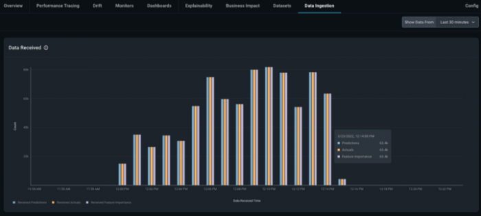
You will be able to see the predictions, actuals, and feature importances that have been sent in the last 30 minutes, day, or week.

An example view of the Data Ingestion tab from a model, when data is sent continuously over 30 minutes, is shown in the image below.

Check the Embedding Data

First, set the baseline to the training set that we logged before.

If your model contains embedding data, you will see it in your Model Overview page.

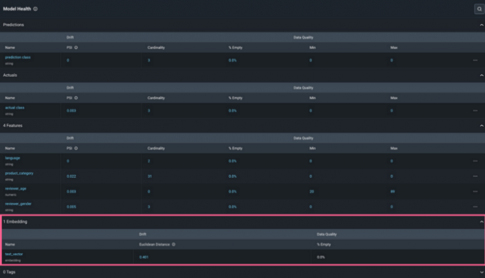
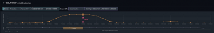
Click on the Embedding Name or the Euclidean Distance value to see how your embedding data is drifting over time. In the picture below, Arize represents the global euclidean distance between your production set (at different points in time) and the baseline (which we set to be our training set). We can see there is a period of a week where suddenly the distance is remarkably higher. This shows that during that time text data sent to our model that was different than what it was trained on (English). This is the period of time when reviews written in Spanish were sent alongside the expected English reviews.

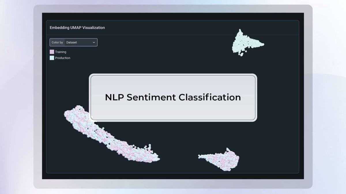
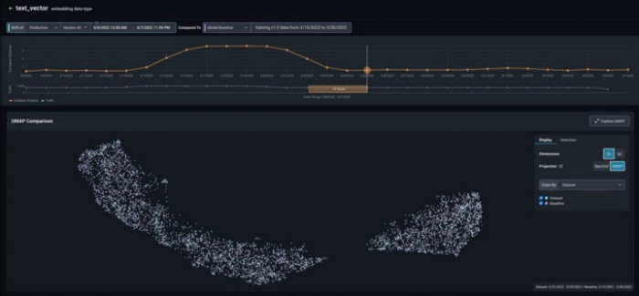
In addition to the drift tracking plot, you can also find the Uniform Manifold Approximation and Projection (UMAP) visualization of your data under the point in time selected. Notice that the production data and our baseline (training) data are superimposed, which is indicative that the model is seeing data in production similar to the data it was trained on.

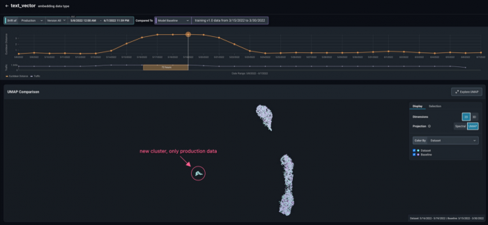
Next, select a point in time when the drift was high and select a UMAP visualization in two dimensions (2D). We can see that both training and production data are superimposed for the most part, but another cluster of production data has appeared. This indicates that the model is seeing data in production qualitatively different to the data it was trained on, and in this case causing performance degradation.

For further inspection, select a three-dimensional (3D) UMAP view and click Explore UMAP to expand the view. With this view, you can interact in 3D with the dataset. Zoom, rotate, and drag to see the areas of the dataset that are most interesting.

In the UMAP display, there are several coloring options that are worth using in different circumstances:

By Dataset: The coloring distinguishes between production data versus baseline data (training in this example). This is specifically useful to detect drift. In this example, we can see that there is some production data far away from any training data, giving an indication of severe dataset drift. We can identify exactly what datapoints our baseline is missing so that re-train effectively.
By Prediction Label: This coloring option gives an insight on how a model is making decisions. Where are the different classes located in the space? Is the model predicting one class in regions where it should be predicting another?
By Actual Label: This coloring option is great for identifying labeling issues. If other colors are visible inside an orange cloud, for instance, it is a good idea to check and see if the labels are wrong. Further, we can use the corrected labels for re-training.
By Correctness: This coloring option offers a quick way of identifying where the bulk of your model’s mistakes are placed, giving you an area to pay attention to. In this example, we can see that the Spanish reviews are almost all red.
By Confusion Matrix: This coloring option allows you to select a positive class and color the data-points as True Positives, True Negatives, False Positives, False Negatives.

Final Note

If you want to remove this example model from your account, just click Models -> NLP-reviews-demo-language-drift -> config -> delete

Conclusion

As teams deploy more NLP sentiment classification models into production, having model monitoring in place to track embedding drift and root cause issues that arise is critical for staying ahead of potential performance degradation in the real world. By taking a few simple steps outlined in this blog, your team can have an easier and more automated way to tackle these challenges head-on!

Questions? Reach out on the Arize community. For additional Colabs, check out the Arize Docs.