This blog was written by Stefano Bosisio

What do we need today?

Firstly, let’s think of the design of the main SDK protocol. The aim today is to allow data scientists to:

1. add to a given experiment’s run the historical metrics computed in previous runs
2. add custom computed metrics to a specific run

Thus, we can think of implementing the two following functions:

1. report_metrics_to_experiment : this function will collect all the metrics from previous experiment’s runs and will group them in an interactive plot, so users can immediately spot issues and understand the overall trend
2. report_custom_metrics : this function returns data scientists’ metrics annotations, posting a dictionary to a given experiment. This may be useful if a data scientist would like to stick to a specific experiment with some metrics on unseen data.

Report experiment runs metrics to the most recent run

This function makes use of the MLflowClient Client in MLflow Tracking manage experiments and their runs. From MLflowClient we can retrieve all the runs for a given experiment. From there, we can extract each run’s metrics. Once we gather together all the metrics we can proceed with a second step, where we are going to use plotly to have an interactive html plot. In this way, users can analyze each single data point for all the runs in the MLflow server artifacts box.

Fig.1 shows the first part of the report_metrics_to_experiment function. Firstly, the MlflowClient is initiated, with the given input tracking_uri . Then, the experiment’s information is retrieved with client.get_experiment_by_name and converted to a dictionary. From here each experiment’s run is listed, runs_list . Each run has its run_id which is practical to store metrics information in a dictionary models_metrics . Additionally, metrics can be accessed via run.to_dictionary()[‘data’][‘metrics’]. This value returns the name of the metric.

Fig.1: First part of the function report_metrics_to_experiment. In this code snippet, I am showing how to retrieve metrics’ data points from the experiment’s runs. The final metrics values are stored in a dictionary, along with the run id, the metric’s steps, and values

From the metric’s name, the metric’s data points can be recorded through client.get_metric_history(). This attribute returns the steps and the values of the metric, so we can append to lists and saved them in models_metrics[single_run_id][metric] = [x_axis, y_axis]

Fig.2 shows the second part ofreport_metrics_to_experiment Firstly, a new plotly figure is initialized fig = go.Figure(). Metrics are then read from models_metrics and added as a scatter plot. The final plot is saved in html format, to have an interactive visualization.

Fig.2: Second part of the function report_metrics_to_experiment. Here all the retrieved metrics are displayed on a plotly plot, which then saved in html format

Report custom metrics to a run

The final function we are going to implement today, reports a custom input to a specific run. In this case, a data scientist may have some metrics obtained from a run’s model with unseen data. This function is shown in fig.3. Given an input dictionary custom_metrics (e.g. {accuracy_on_datasetXYZ: 0.98} ) the function uses MlflowClient to log_metric for a specific run_id

Fig.3: report_custom_metrics take an input dictionary, with unseen metrics or data, and it reports the key and val to the MLflow run with log_metric.

Update the experiment tracking interface

Now that two news functions have been added to the main MLflow protocol, let’s encapsulate them in ourexperiment_tracking_training.py In particular, end_training_job could call report_metrics_to_experiment , so, at the end of any training, we can keep track of all the historical metrics for a given experiment, as shown in fig.4

Fig.4: report_metrics_to_experiment can be called at the end of any training job and added to the end_training_job functionality.

Additionally, to allow users to add their own metrics to specific runs, we can think of an add_metrics_to_run function, which receives as input the experiment tracking parameters, the run_id we want to work on, and the custom dictionary custom_metrics (fig.5):

Fig.5: Custom metrics can be reported through experiment_tracking_training.add_metrics_to_run module.

Create your final MLflow SDK and install it

Patching all the pieces together, the SDK package should be structured in a similar way:

The requirements.txt contains all the packages we need to install our SDK, in particular, you’ll neednumpy, mlflow, pandas, matplotlib, scikit_learn, seaborn, plotly as default.

setup.py allows you to install your own MLflow SDK in a given Python environment and the script should be structured in this way:

Fig.6: Setup.py to install our mlflow_sdk package in a given Python environment

To install the SDK just use Python or a virtualenv Python as python setup.py install

SDK in action!

It’s time to put into action our MLflow SDK. We’ll test it with a sklearn.ensemble.RandomForestClassifierand the iris dataset¹ ² ³ ⁴ ⁵ (source and license, Open Data Commons Public Domain Dedication and License). Fig.7 shows the full example script we are going to use (my script name is 1_iris_random_forest.py)

tracking_params contains all the relevant info for setting up the MLflow server, as well as the run and experiment name. After loading the dataset, we are going to create a train test split with sklearn.model_selection.train_test_split . To show different metrics and plots in the MLflow artifacts I run 1_iris_random_forest.py 5 times, varying the test_size with the following values:0.3, 0.2, 0.1, 0.05, 0.01

Fig.7: In the example, we are going to run a random forest against the iris dataset. The MLflow SDK will keep track of the model info during training and report all the additional metrics with add_metrics_to_run.

Once the data have been set up, clf=RandomForestClassifier(n_estimators=2) we can call experiment_tracking_training.start_training_job. This module will interact with the MLflow context manager and it will report to the MLflow server the script that is running the model as well as the model’s info and artifacts.

At the end of the training, we want to report all the experiment run’s metrics in a single plot and, just for testing, we are going to save also some “fake” metrics like false_metrics = {“test_metric1”:0.98, … }

Before running the 1_iris_random_forest.pyin a new terminal tab open up the connection with the MLflow server as mlflow ui and navigate to http://localhost:5000 orhttp://127.0.0.1:5000 . Then, run the example above aspython 1_iris_random_forest.py and repeat the run 5 times for different values of test_size

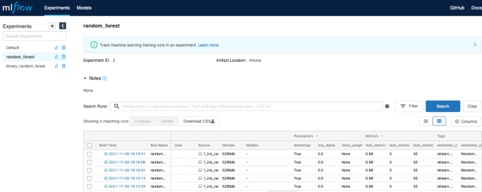
Fig.8: MLflow UI after running the example script

Fig.8 should be similar to what you have after running the example script. Under Experiments the experiments’ names are listed. For each experiment there is a series of runs, in particular, under random_forest you’ll find your random forest runs, from 1_iris_random_forest.py

For each run we can immediately see some parameters, which are automatically logged by mlflow.sklearn.autolog() as well as our fake metrics (e.g. test_metric1 ) The autolog function saves also Tags , reporting the estimator class (e.g. sklearn.ensemble._forest.RandomForestClassifier) and method ( RandomForestClassifier ).

Clicking on a single run more details are shown. At first, you’ll see all the model parameters, which, again, are automatically reported by the autolog function. Scrolling down the page we can access the Metrics plots. In this case, we have just a single data point, but you can have a full plot as a function of the number of steps for more complicated models.

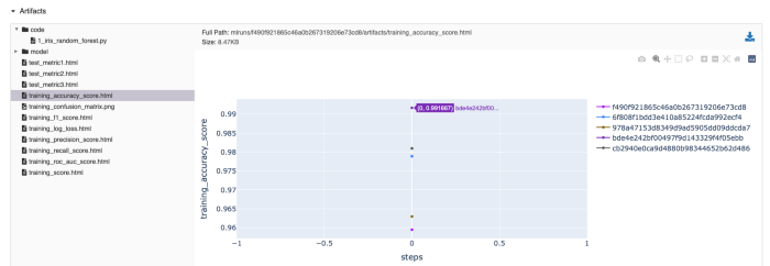
Fig.9: Artifacts saved by MLflow SDK. In the artifacts box, you can find the code used to run the model (in my case 1_iris_random_forest.py) as well as the model pickle files under model folder and all the interactive metrics plots as well as the confusion matrix.

The most important information will then be stored under the Artifacts box (fig.9). Here you can find different folders which have been created by our mlflow_sdk:

1. Firstly, code is a folder that stores the script used to run our model — this was done in experiment_tracking_training on line 24 with traceback , here the link, and pushed to MLflow artifacts on line 31 of run_training function, here the link).
2. Following, model stores binary pickle files. MLflow automatically saves model files as well as their requirements to allow the reproducibility of the results. This will be super helpful at deployment time.
3. Finally, you’ll see all the interactive plots. ( *.html ), generated at the end of the training, as well as additional metrics we have computed during the training, such as training_confusion_matrix.png

As you can see, with minimal intervention we have added a full tracking routing to our ML models. Experimenting is crucial at development time and in this way, data scientists could easily use MLflow Tracking functionality without over-modifying their existing codes. From here you can explore different “shades” of reports, adding further information for each run as well as running MLflow on a dedicated server to allow cross-team collaboration.

Author’s Bio: Stefano is a Machine Learning Engineer at Trustpilot, based in Edinburgh. Stefano helps data science teams to have a smooth journey from model prototyping to model deployment. Stefano’s background is Biomedical Engineering (Polytechnic of Milan) and a Ph.D in Computational Chemistry (University of Edinburgh).