Query Multiple Documents using LlamaIndex, LangChain, and Milvus

Large Language Models (LLMs) are popular for personal projects, but how can we use them in production? One of the immediate use cases that stands out is using an LLM like GPT to query your documents. It’s not enough to query one document; instead, we need to query multiple documents. LlamaIndex and Milvus can help us get started in a Jupyter Notebook. Here is a link to the CoLab Notebook.

In this tutorial, we cover:

1. Setting Up Your Jupyter Notebook for Multiple Document Querying

1. Building Your Document Query Engine with LlamaIndex

1. Starting the Vector Database
2. Gathering Documents
3. Creating Your Document Indices in LlamaIndex
4. Decomposable Querying Over Your Documents

1. Comparison with Non-Decomposed Queries

1. Summary of How to Do Multi-Document Querying Using LlamaIndex

Setting Up Your Jupyter Notebook for Multiple Document Querying

To get started, we need to set up our libraries. We need seven libraries to run this code: `llama-index`, `nltk`, `milvus`, `pymilvus`, `langchain`, `python-dotenv`, and `openai`. The `llama-index`, `nltk`, `langchain`, and `openai` libraries help us connect to an LLM to perform our queries.

The `pymilvus` and `milvus` libraries are for our vector database and `python-dotenv` is for managing our environment variables. We also need to set up NLTK before we can create decomposable queries. The code below shows how to download the `stopwords` module from NLTK and code to get around a common SSL error that comes up.

Building Your Document Query Engine with LlamaIndex

Now that we’ve set up our Jupyter Notebook, it’s time to build the Document Query Engine. There are a lot of imports here. First, we need two indices: a vector index and a keyword table index. Second, we need the `SimpleDirectoryReader` to read data from a directory.

Third, we need a way to use the LLM. For this, we use `LLMPredictor`. Fourth, we need two contexts: a service context and a storage context. These are the basic LlamaIndex imports for now, we have a few more down the line in the Jupyter Notebook as we continue. Finally, we also need to import the OpenAIChat tool from LangChain.

The last step to get our notebook ready to build a mini LLM application is getting our LLM access. I’ve loaded my OpenAI API key, which you can get from their website, in a `.env` file. I use `load_dotenv()` to load the `.env` file and then set the `api_key` parameter of `openai` to the loaded key.

Starting the Vector Database

Once we have our notebook setup, it’s time to start putting the code for the working parts of the app together. Step one is to spin up a vector database. We need the actual vector database server from `milvus` and the `MilvusVectorStore` class from LlamaIndex. We need to start the `default_server` and connect to it using the `MilvusVectorStore` object passing in the host (localhost) and the port.

Gathering Documents

Let’s get the documents that we are querying over. For this example, we will learn about some big cities from Wikipedia. We will use Wikipedia articles about Toronto, Seattle, San Francisco, Chicago, Boston, Washington DC, Cambridge (Massachusetts), and Houston.

We use the `requests` library to get the Wikipedia docs. Start by creating a for loop to loop through all the list titles. Then, for each of these titles, send a `GET` request to the Wikipedia API. We need five parameters for each request: `action`, `format`, `titles`, `prop`, and `explaintext`.

All of the text from the Wikipedia article is under the `extract` key. So, we compile all the pages together and load that into one variable containing all the text. Then, with all of our text in hand, we write the files to a local folder and give them each the right titles.

Creating Your Document Indices in LlamaIndex

Now that we have all the data, it is time to bring in LlamaIndex to create our indices to search through them. Start by creating an empty dictionary to hold all the documents about the cities. Then, loop through each of the titles from above and read in the file.

Next, we instantiate the LLM Predictor. We’ll use GPT 3.5 Turbo through LangChain’s `OpenAIChat` object for this. We also need to create two contexts for our index: a service context and a storage context. We create the service context from the LLM predictor model and the storage context from the Milvus vector store we made earlier.

The next step is to create two empty dictionaries for the city indices and the summaries. Once again, we loop through the cities we chose above. This time, we create a `GPTVectorStoreIndex` object from each of the docs we read in earlier, save it to the city index, and save a meta description to the summary dictionary.

Decomposable Querying Over Your Documents

The key to comparing and contrasting multiple documents is using a “decomposable query.” A decomposable query is a query that we can break down into smaller parts. First, we import the `ComposableGraph` object from LlamaIndex. Then, we create a composable graph from some indices.

In this example, we use a Keyword Table Index, the list of indices from the city indices, and the list of indices from the “summary” indices. We can also provide a parameter for the maximum number of keywords in a chunk; for this example, we use 50. Next, we import the `DecomposeQueryTransform` object and create an object that can transform and decompose queries using the ChatGPT LLM Predictor we created earlier.

Next, we create the engines to do the query transformation. To do this, we first import `TransformQueryEngine`. Then, we need another empty dictionary to hold the query engine mappings. Next, we loop through each of the indices in the city indices.

We create a query engine for each of these indices using the index `as_query_engine`. We also add some extra information through the summary index we created. Finally, we feed the index as a query engine and the summary index as extra info into the `TransformQueryEngine` object and the `DecomposeQueryTransform` object from above to create a custom query engine.

There is still one more set of custom query engines to create. We add the root of the decomposable graph we created above as an entry and use it in summarization mode. Finally, we create a query engine from the graph that uses the dictionary of custom query engines we created above.

Now we are ready to query over all of these documents. In this example, we ask our LLM app to compare and contrast the Seattle, Houston, and Toronto airports. Earlier we made our query decomposition verbose so we can see how our app is decomposing the query.

The image below is the decomposition of our query. It shows asking about the airports in Seattle, Houston, and Toronto.

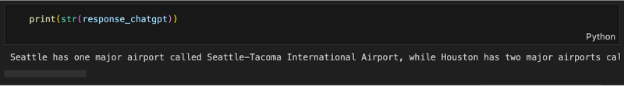
The image below shows part of the response. The complete response is “Seattle has one major airport called Seattle-Tacoma International Airport, while Houston has two major airports called George Bush Intercontinental Airport and William P. Hobby Airport, as well as a third municipal airport called Ellington Airport. Toronto’s busiest airport is called Toronto Pearson International Airport and is located on the city’s western boundary with Mississauga. It offers limited commercial and passenger service to nearby destinations in Canada and the United States. Seattle-Tacoma International Airport and George Bush Intercontinental Airport are major international airports, while William P. Hobby Airport and Ellington Airport are smaller and serve more regional destinations. Toronto Pearson International Airport is Canada’s busiest airport and offers a direct link to Union Station through the Union Pearson Express train service.”

Comparison with Non-Decomposed Queries

Why do we need decomposable queries to query over multiple documents? Because finding and gathering data from various sources requires the LLM application to split and route queries to the right source. Imagine if you asked a New Yorker who has never been to LA about LAX. What could they tell you? Next to nothing.

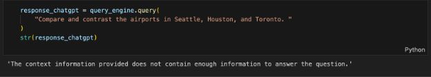
Let’s look at what would happen if we didn’t use a decomposable query. The code below remakes the custom query engine with one main difference. We don’t add in the query transformer (or the extra “summary” info required) when making the city indices.

When we query with this query engine, we get a response that tells us the provided contextual information (the documents) don’t have enough information to answer the question. That’s because if we don’t break it down, we are in essence, asking someone who has only been to the Seattle airport to compare it to the airports in two cities she has not been to.

Summary of How to Do Multi-Document Querying Using LlamaIndex

This tutorial taught us how to make a question-answer app over multiple documents in your iPython Notebook using the “LLM” stack – LlamaIndex, LangChain, and Milvus. The Q/A app uses the concept of decomposable queries and stacks a vector store index with a keyword index to handle splitting and routing queries correctly in LlamaIndex.

Query decomposition allows us to break down complex queries into simpler, targeted ones. A keyword index will enable us to route the queries through keyword searches. Finally, a vector store index allows us to process semantic information. Putting all of this together, we can answer a question that requires information from many sources.

First, the transformer breaks the question into simple queries that a single data source can answer. Then, it uses the keyword index to route the simple queries to the right data source and the vector store index to answer the question. Finally, the question transformer combines the information and answers our original, complex query.